Subscribe to
Posts
Comments

I’m pleased to announce the availability of version 0.2 of my criterion library for Haskell performance evaluation.

Compared to version 0.1, this version has some significant changes.

  • The benchmarking API has been improved! If you’re benchmarking a pure function, you no longer need to feed it an Int to ensure that it won’t get thunked or let-floated. Instead, Use the B data type (see the examples/ directory) to specify an unsaturated function that you want to benchmark, along with its last argument. Many thanks to Daniel Peebles for suggesting this approach, which makes the use of criterion considerably more pleasant.
  • Neil Brown added a --kde-same-axis command-line option to allow plotting the KDEs for all the benchmarks with the same X axis. I’d like to thank Neil for his helpful work on some other code cleanup issues, too.
  • There are some more, and better quality, examples in the examples/ directory.
  • Tim Docker contributed a patch that improves graph rendering.

As the changes above suggest, several people have been actively contributing to the improvement of criterion, and I’m delighted by this. Please feel welcome to get involved; there are many improvements I’d like to make, but of course I have limited time to work on them. I’ll be happy to talk with you about other potentially useful changes.

I'm pleased to announce the availability of version 0.5 of text, a library that provides fast Unicode text handling for Haskell.

This version contains numerous changes compared to version 0.4, in three broad categories:

  • I made improvements to the performance of some common functions by, in many cases, more than 10x.

  • I have substantially refined the API.

  • Many bugs fixed, almost all of them subtle, thanks to the ever-astounding QuickCheck library.

Performance improvements

In real-world code, many of the most frequently performed text manipulation operations involve searching for substrings. I've written a fast search function, based on Fredrik Lundh's very elegant adaptation of the Boyer-Moore-Horspool-Sunday algorithm, and rewritten all of the functions that perform searches internally to use it (without changing any of the APIs in question, of course).

Retooling with this function has made a big difference to performance. Here are measurements of old-style searches, searches over the popular ByteString type, and new-style searches:

big slow densities

big bytestring densities

big fast densities

For this data set, the new search code is 10.4 times faster than the old, and 24% faster than the ByteString search code.

If we perform a search for a short snippet of DNA in a large data set, we see a similar pattern:

dna slow densities

dna bytestring densities

dna fast densities

Over the DNA data set, the new search code is 15.3 times faster than the old, and 85% faster than the ByteString search code.

By the way, it was writing—and wanting to measure the performance of—this new search function that led me to create the criterion benchmarking package, which in turn begat the statistics package. What a month of hacking it's been!

API changes

While the API of the text package still somewhat resembles the venerable Data.List API (which is now almost two decades old), I have modified it to be both narrower and more useful for text processing tasks.

All of the integer-index-based search functions are now gone, since using integer offsets into Unicode strings is a bad idea (especially when the underlying representation uses a variable-length encoding).

Instead, the search functions break up the original string. Consider the new find function, for instance:

find :: Text -> Text -> (Text, [(Text, Text)])

This function returns all non-overlapping instances of needle in haystack. The first element of the returned pair is the prefix of haystack prior to any matches of needle. The second is a list of pairs.

The first element of each pair in the list is a span from the beginning of a match to the beginning of the next match, while the second is a span from the beginning of the match to the end of the input.

find "::" ""
==> ("", [])

find "/" "a/b/c/d"
==> ("a", [("/b","/b/c/d"), ("/c","/c/d"), ("/d","/d")])

Notice that no matter how much of the result list you consume, you can always reconstruct the entire original haystack from the elements you've already seen.

More often, you won't want something nearly this general. Instead, you may want a function that simply splits a string on a separator:

split :: Text -> Text -> [Text]

Here are a few examples of how the split function works:

split "\r\n" "a\r\nb\r\nd\r\ne"
==> ["a","b","d","e"]

split "aaa" "aaaXaaaXaaaXaaa"
==> ["","X","X","X",""]

split "x" "x"
==> ["",""]

Some of the functions supplied by the list API are not very useful in the context of a text-oriented API. Consider break:

break :: (a -> Bool) -> [a] -> ([a],[a])

I use this name in the text package, but give the function a simpler and more useful type signature (its behaviour is otherwise the same):

break :: Text -> Text -> (Text, Text)

If, for some reason, you still want the predicate-based functions, they're usually available, but (in most cases) with a "By" suffix added, to provide uniform naming:

breakBy :: (Char -> Bool) -> Text -> (Text, Text)

Testing and bug fixes

Even though the text package already had a very high degree of test coverage, I still found perhaps a dozen bugs while working on this release. The bugs in question were almost without exception quite subtle, and it would have been tremendously difficult to reproduce them, or to fix them with confidence, without the assistance of the QuickCheck library.

By the way, even though I've been using it for years, I still find myself feeling very strongly that the QuickCheck library is simply amazing. If unit testing is like riding a tricycle with wobbly wheels, working with QuickCheck more closely resembles flying a sleek starship. Wow.

At the moment, the profile of code covered by QuickCheck tests looks like this:

  • 96% of public top-level definitions

  • 85% of conditional expressions

  • 88% of all expressions

(In case you're wondering, these are higher levels of test coverage than those achieved by the widely used bytestring package, so you should have high confidence that the code in the text package is pretty solid.)

And has prettier charts, too, thanks to a patch from Tim Docker.

If you already have criterion installed:

$ cabal update
$ cabal install --reinstall criterion

If you want to use criterion on a Mac:

$ cabal update
$ cabal install criterion -f-chart

Alas, on OS X, you’ll lack the ability to directly generate pretty chart images, but criterion will still output CSV files for you. You can import these into gnuplot or your favourite spreadsheet with ease, and chart away from there.

I'm pleased to announce the availability of criterion, a new library for measuring the performance of Haskell code.

Compared to most other benchmarking frameworks (for any programming language, not just Haskell), criterion focuses on being easy to use, informative, and robust.

Here's a canonical benchmark-worthy function, which has the desirable properties of being both small and slow:

-- Save this as a file named "Fibber.hs".

import Criterion.Main (defaultMain)

fib :: Int -> Int
fib 0 = 0
fib 1 = 1
fib n = fib (n-1) + fib (n-2)

To compile a program that will benchmark our fib function, we write a trivial main entry point:

-- Append this to the end of "Fibber.hs".

main = defaultMain [
bench "fib 10" $ \n -> fib (10+n-n)
, bench "fib 30" $ \n -> fib (30+n-n)
, bench "fib 35" $ \n -> fib (35+n-n)
]

Criterion itself is trivially easy to install.

$ cabal install criterion

Once it's installed, we build the application we intend to benchmark.

$ ghc -O --make Fibber

If we run the Fibber program with the --help option, it prints a large amount of help output. The most interesting options early on are -t, which displays raw timing information, and -k, which turns the timing information into a chart of the probability distributions of timings. So for immediate gratification, we can run Fibber like this:

$ ./Fibber -t win -k win

The win argument to each option means "display these charts in a window". For this article, I used the png argument instead, to get nicely sized images that I could simply drop into Wordpress.

$ ./Fibber -t png:450x175 -k png:450x175

Here's an example of raw timing information:

fib 10 timings

Notice that the times on the Y axis are labelled with their units, in this case microseconds. On the X axis is the run count.

Timing information is somewhat nice to have, but much more useful is an indication of which times occurred most frequently. The traditional way to display such information is with a histogram. Histograms are pretty awful, since a histogram with an incorrect bin size is either misleading or useless, and bin sizes have to be chosen by hand. Much more useful is a kernel density estimate:

fib 10 densities

This is a chart of the estimated probability densities of timings. We observe a big hump at about 5.23µs, with a few small outliers further out. This suggests that it usually takes about 5.23µs to evaluate fib 10.

Meanwhile, in our console window, our Fibber program has printed a lot more information. Here's how it starts:

estimating clock resolution...
mean is 9.956511 us (80001 iterations)
found 3711 outliers among 79999 samples (4.6%)
  3505 (4.4%) high severe

The first thing that Fibber does is measure how long it takes for the system clock to tick. It will then run our benchmarked code enough times that the resolution of the clock will not introduce a significant error.

Indeed, our first benchmark shows why this is important: if fib 10 takes 5.23µs to evaluate, but the clock ticks once every 9.96µs, we clearly can't just evaluate fib 10 once, and subtract the start from the end time. Sometimes it will appear to evaluate instantaneously, since the clock won't have ticked, and sometimes it will appear to have taken about 10µs, since the clock will have ticked exactly once. Both answers would be worse than useless.

Instead, we evaluate fib 10 many thousands of times in order to get the measurement error introduced by the resolution of the clock down to a few parts in ten thousand.

We also use something called the boxplot technique to develop a quick sense of the quality of our data. In this case, a few percent of our numbers are significantly off from the mean of the sample.

Once we've characterised the system clock's period, we figure out how expensive it is to actually use the clock.

estimating cost of a clock call...
mean is 923.3224 ns (58 iterations)
found 4 outliers among 58 samples (6.9%)
  1 (1.7%) high mild
  3 (5.2%) high severe

We adjust our timing measurements to take the cost of clock calls into account, even though in practice this makes almost no difference to the numbers we report. (If you're measuring an event that occurs on a millisecond-to-second time scale, you wouldn't expect a one-microsecond difference to perturb things much!)

The last part is the most interesting. We automatically figure out how many times we need to evaluate fib 10:

benchmarking fib 10
collecting 100 samples, 1911 iterations each, in estimated 995.8188 ms

In this case, we evaluate fib 10 1911 times and measure the cost of this, then repeat this measurement 100 times. We print an estimate in advance for how long the measurements will take, so that if you're benchmarking something expensive, you can go for coffee or whatever. (If you can fetch coffee in 995.8 milliseconds, more power to you!)

Why do we measure so many times? Because we're going to do some statistical analysis of our measurements to see whether they are trustworthy.

bootstrapping with 100000 resamples

The bootstrap step takes a second or two, and this is where the interesting stuff takes place. The performance of real-world applications doesn't follow some kind of tidy statistical pattern such as the normal distribution, especially when people are measuring in realistic, noisy environments.

If you run a time-consuming benchmark on your laptop, you're likely to want to switch to your web browser, watch a video on youtube, check your mail, and so on. Your CPU might slow down because it's overheating, or your laptop's ACPI subsystem might change the CPU frequency to conserve power.

In other words, there are lots of things that might perturb our benchmarking results, some of which we can't see or control, but then again they might not occur or might not be important, and our numbers could be fine. How can we tell?

We use a statistical technique known as the bootstrap, with which we take some sample data and perform some number crunching to tell us interesting things. Specifically, we can use the results of the bootstrap to tell us whether the outliers in our measurements (timings that are far from the mean) are perturbing our numbers in a significant way.

The first thing that the bootstrap tells us is the mean and standard deviation of our measurements, along with the 95% confidence intervals for those values.

mean: 5.232800 us, lb 5.222862 us, ub 5.262482 us, ci 0.950
std dev: 79.86726 ns, lb 31.06332 ns, ub 173.0716 ns, ci 0.950

It then reports on the outliers in the measurements, and most importantly, tells us whether they are important.

found 7 outliers among 100 samples (7.0%)
  3 (3.0%) high mild
  4 (4.0%) high severe
variance introduced by outliers: 0.993%
variance is unaffected by outliers

I ran the above example on my laptop when it was idle, so the timing measurements are fine. Boring!

What about a more interesting example? I measured the performance of fib 35:

collecting 100 samples, 1 iterations each, in estimated 88.14368 s

While this executed, I ran a stupid but computationally expensive task in another window:

while true; do
  for ((i=0;i<20;i++)); do
    md5sum cufp.odp >/dev/null &
  done
  for ((i=0;i<20;i++)); do
    wait
  done
done

This shell script grinds over a largish file repeatedly, but does so using 20 processes at a time. It reliably drives the load average on my laptop up to 8. What did it do to my measurements?

fib 35 timings

As the timing numbers suggest, I ran my CPU-chomping script twice while taking measurements. This had a noticeable effect not just on the timings, but on their probability distributions too:

fib 35 densities

Those are two fairly large humps, which certainly seem like they should give cause for concern. What does Fibber report on the console?

mean: 1.566470 s, lb 1.333717 s, ub 1.855111 s, ci 0.950
std dev: 1.324608 s, lb 1.114684 s, ub 1.510580 s, ci 0.950
found 23 outliers among 100 samples (23.0%)
  22 (22.0%) high severe
variance introduced by outliers: 52.994%
variance is severely inflated by outliers

Notice that the standard deviation of the sample is almost the same as the mean, a classic sign of sketchy performance measurements. However, we don't merely have to spot this suspicious pattern ourselves: by analysing the results of the bootstrap, our benchmark automatically tells us that our numbers are, in effect, junk.

So! Thanks to criterion, you can now easily measure the performance of Haskell code, and even better, you'll (usually) be told when you're lying to yourself. Oh, and you can produce those charts in PDF, SVG, and CSV formats, too, in addition to PNG and windowed output, so you can simply drop camera-ready copy straight into your next Haskell Implementor's Workshop submission!

There's plenty of work yet to be done. In order to improve the rigour of the bootstrap analysis, I want to perform an autocorrelation test on the timing measurements, since an autocorrelated sample can distort the result of a bootstrap analysis. I'd also like to be able to produce charts with many estimates overlaid, to allow things like scaling and comparative analyses. But I think that criterion is off to a solid start. If you'd like to work on any of these, let me know: I think that the code is quite clean and easy to work on, and of course the darcs repository for the source is easy to get:

darcs get http://darcs.serpentine.com/criterion

It should even be easy to use criterion to benchmark C code and command line programs.

Much of my work on criterion was inspired by Brent Boyer's excellent articles on Java performance analysis (part one and part two). Amusingly, Java and Haskell each pose substantial benchmarking challenges: in the case of Java, dynamic recompilation makes getting good numbers very challenging, while for Haskell, lazy evaluation brings its own difficulties.

Riddle me this

I find Lennart Augustsson's Text.Printf module very handy, but also quite baffling.

Here is one example of my bafflement: suppose I want to print a piece of text if my program's verbosity level is above a certain threshold, but not otherwise. I'd like to hide that detail in a function, such that I could just call something like this:

 note cfg "mean is %s (%d iterations)\n" (secs µ) iters

and my note function would Do The Right Thing. The type signature of hPrintf seems to make this impossible to do elegantly, since the number of arguments to note is not clear. Hence a fugly hack:

nullDev :: Handle
nullDev = unsafePerformIO $ openBinaryFile "/dev/null" WriteMode
{-# NOINLINE nullDev #-}

note :: (HPrintfType r) => Config -> String -> r
note cfg msg = if cfgVerbosity cfg > Quiet
               then hPrintf stdout msg
               else hPrintf nullDev msg

This makes me a sad Irish panda.

The next thing I'd like to be able to do, and over which I am also baffled, is to hide that Config parameter, since it's ubiquitous in my code:

newtype Criterion a = Criterion (ReaderT Config IO a)
    deriving (Monad, MonadReader Config, MonadIO)

Most of the time, I can ask for the current Config when I need to. However, when it comes to eliminating this parameter from my note function, I am once again stymied by the type of hPrintf, since there's no way to tell what monad I'm living in.

Help!

Video of my CUFP keynote

Thanks to the tireless work of Malcolm Wallace, all of the video from CUFP now appears to be up up Vimeo, including the keynote talk I gave.

Keynote: Real world Haskell. from Malcolm Wallace on Vimeo.

I just released version 0.3.3 of the Haskell statistics library, which contains a very fast pseudo-random number generator.

The generator is an implementation of George Marsaglia’s MWC256 multiply-with-carry PRNG, which has a period of 28222 (for this reason, it’s sometimes referred to as MWC8222). It produces high-quality uniformly distributed pseudo-random numbers extremely quickly.

Here is a brief performance comparison between the statistics library, the mersenne-random library, the normal Haskell PRNG, and a C implementation of MWC256. The numbers represent millions of variates generated and summed per second, so higher is better. (Measured on a 64-bit Core2 Duo laptop running Fedora 11.)

Package Int64 Double Word32
System.Random 0.7 1.6 n/a
mersenne-random 101.2 53.8 96.3
statistics 145.7 116.5 251.6
C (normal) 131.0 103.2 292.9
C (inlined) 162.0 118.7 375.6
C (inlined, unrolled) 186.5 171.7 571.2

As the numbers indicate, the MWC256 implementation in the statistics library is up to 3 times faster than the mersenne-random library, and often faster than the C code you’d expect to encounter in practice. And you shouldn’t use the standard Haskell PRNG if you care about performance.

(The last two rows in the table above indicate what you could expect from an aggressive C compiler that performed cross-module inlining and loop unrolling, such as almost works reliably in gcc these days. If you were using normal compilation flags and source file structure, you would be unlikely to see those kinds of numbers in practice.)

A nice feature of the PRNG in the statistics library is that it has a cleaner interface than mersenne-random. Due to the cheesy implementation of the underlying C code, the mersenne-random library enforces the use of a single PRNG for the entire program, which makes it onerous to work with. You have to create a single generator when your program starts, and pass it everywhere that you might eventually need random numbers. In a multi-threaded program, only one thread at a time can use the PRNG.

The PRNG in the statistics library runs inside the ST monad, so you can generate random variates from inside pure Haskell code. You can create or use a generator anywhere without worrying about threading issues, and there’s a handy function provided that lets you seed a generator from your system’s random number source.

As a final tweak, the new PRNG generates floating point numbers in the range (0,1], so the variates it generates are safe for using in statistical computations that are zero-phobic, such as those involving logarithms or division. I’ve also included a generator for normally-distributed floating point numbers that uses Doornik’s modified ziggurat algorithm, so it’s both fast and trustworthy.

Malcolm Wallace has very kindly put a lot of work into publishing video footage from all of the talks at last week’s Haskell Implementor’s Workshop. I gave a very brief, and completely unscripted, demo of the benchmarking framework that I’ve been hacking on. This was code that I’d literally gotten working about 45 minutes before I started speaking, so it was quite the seat-of-my-pants experience. Lots of fun!

Statistical benchmarking in Haskell from Malcolm Wallace on Vimeo.

A few weeks ago, I decided that I'd like to focus for a while on getting a 1.0 release of the Haskell text library ready. That work has gone fairly well so far. I've focused on making sure that I like the API, and that a few key functions have good performance characteristics.

One such function is substring search, which is the underpinning for a number of useful functions (split a string on a delimiter, find all substrings, etc). My initial cut at that function had an obvious API, but ran in O(nm) time, which complexity measure I found mildly embarrassing. So I looked around for an alternative that would be faster, but still simple to implement, and settled upon Fredrik Lundh's elegant and trim adaptation of Boyer-Moore-Sunday-Horspool, which has O(n+m) complexity in the typical case.

Using QuickCheck, I was quickly able to satisfy myself that my new code was correct, so now I was faced with demonstrating to myself that the code was fast, too. I looked on Hackage for a good benchmarking package, but although there were several benchmarking packages available, they were all extremely simple, and I wasn't happy with any of them.

I have sort of a mutt's pedigree in computing, having spent several stints working in the high performance scientific computing world, so I felt antsy about measuring performance reliably. Over the course of a few days of hacking, I came up with a good framework that I am currently finishing off.

One of the things a good benchmarking framework needs is some statistical heavy lifting, to do things like autocorrelation analysis, kernel density function estimation, and bootstrapping, so I had to write some complicated statistical code along the way. I've now packaged that code up and released it as the statistics library on Hackage. Some of the features implemented in this first release of the statistics library include:

  • Support for common discrete and continuous probability distributions (binomial, gamma, exponential, geometric, hypergeometric, normal, and Poisson)
  • Kernel density estimation
  • Autocorrelation analysis
  • Functions over sample data
  • Quantile estimation
  • Resampling techniques: jackknife and bootstrap estimation

The statistics library certainly isn't yet comprehensive, but it has some features that I think make it very attractive as a base for further work:

  • It's very fast, building on some of the fantastic software that's available on Hackage these days. I make heavy use of Don Stewart's uvector library (itself a port of Roman Leshchinskiy's vector library), which means that many functions allocate no memory and execute tight loops using only machine registers. I use Dan Doel's uvector-algorithms library to perform fast partial sorts. I also use Don's mersenne-random library for fast random number generation when doing bootstrap analysis.
  • I've put a fair amount of effort into finding and using algorithms that are numerically stable (trying to avoid problems like catastrophic cancellation). Whenever possible, I indicate which methods are used in the documentation. (For more information on numerical stability, see What Every Scientist Should Know About Floating-Point Arithmetic).

For me, one of the killer features of Haskell for statistical computation is its combination of terseness and fabulous libraries. In particular, the modern collection libraries like uvector and text, which are built on stream fusion frameworks, provide a combination of expressiveness and high performance that is simply delightful to work with.

Speaking of improving the statistics library, I've already received a few patches to the statistics library even before announcing it anywhere, and I'm very much looking forward to receiving more. If you want to contribute, go get the source code and hack away:

darcs get http://darcs.serpentine.com/statistics

So now that the statistics library is in good enough shape, I can return to work on the benchmarking framework. Once that's done, I'll get back to finishing off the text library. It's been funny to see how rewriting 50 lines of code has spawned off weeks of enjoyable work on other projects! I hope that people will find all of this work useful.

By the way, the philosophy underlying the text, statistics, and benchmarking libraries is uniform across the lot of them: build and release something that—even though initially incomplete—is thorough enough and of such high quality that other people will be drawn to improving your work instead of creating half a dozen tiny alternatives. So please, join in, and let the patches fly!

Several months ago, I wrote an article on evaluating revision control systems. It was initially published in ACM Queue a few weeks ago, and the article has now made its way (unchanged) to Communications of the ACM. I’m quite happy with how it turned out, and I hope that people will find it useful in figuring out what’s important to them.

Since the publication of the article, a few people have asked why I didn’t write about their favourite revision control system. The simple answer is that I was already about 50% over my initial word budget by the time I finished up what I did write. (I’ll confess that I was thoroughly charmed by a conspiratorial suggestion that I was editing some beloved tool out of history by not mentioning it.)

« Prev - Next »